SURVEY GEOMETRY


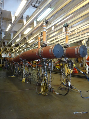
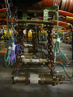
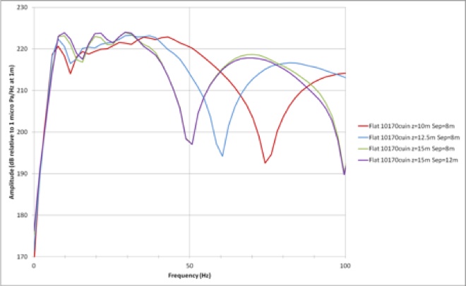
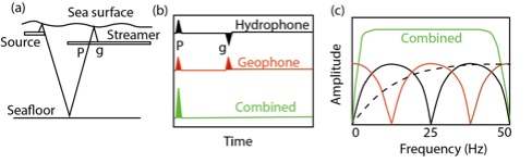
The ultra-deep reflection part of the TransAtlanticILab experiment took place in March-April 2015, on board the WesternGeco seismic vessel Western Trident. A 12 km long IsoMetrix streamer was deployed at 30 m water depth. The energy source was 10170 cubic inches, air-gun array comprised of 6 sub-arrays with 8 guns each, deployed at 15 m depth, providing very low frequency. The 12 km IsoMetrix streamer contained a pressure sensor and three-component accelerometer sensors at the same location. The shot interval varied from 50 m to 75 m, and consequently the record length from 20 s to 30 s, depending upon the target depth along the profile. 

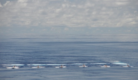
A total of 2775 km ultra-deep seismic reflection data was acquired starting from Greenwich Meridian at 1º S, at about 75 Ma of oceanic lithosphere (Figure 2) in nearly E-W direction, crossing the Mid-Atlantic Ridge at 1.3º S, corresponding to zero age of the lithosphere. This part of the profile spans 0-75 Ma of the oceanic lithosphere on the African Plate. The profile extends ~500 km west of the Mid-Atlantic Ridge and transects 0-25 Ma of the oceanic lithosphere on the South American Plate. 

This E-W profile is connected with an N-S profile that traverses the Chain Fracture Zone, Romanche Transform Fault and St Paul Fracture Zone. These fracture zones are responsible for the shape of Equatorial Africa and Brazil and the 2000 km E-W coastline along the Equatorial Africa.  

The age contrast across the Chain Facture Zone is about 15 Ma, i.e. an offset 300 km; across the Romanche Transform Fault the age contrast is 45 Ma, with an offset of 900 km, and across St. Paul it is 35 Ma with an offset of 700 km. The Romanche transform fault is largest transform fault on Earth and has hosted series of large earthquakes, including the 1994 Mw=7.1 earthquake. It is ~40 km wide, and consists of a deep valley reaching to a water depth of 6200 m along our profile, bounded by ridges that rise up to 1700 m below the sea surface.

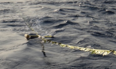
Being in the equatorial region, barnacle growth on the streamer and strong current were two major problems. The barnacle growth created noise on acceleration data and increased the tension on the streamer, slowing down the vessel speed. The streamer needed to be cleaned twice during the16 days of acquisition. Since the streamer was towed at 30 m, the current at this depth was often in the opposite sense to that on the surface, usually much stronger, further reducing the speed, some times down to 3 knots.

STREAMER


     IsoMetrix System


The IsoMetrix* streamer consists of two pressure sensors, and 3-component acceleration sensors (Ax, Az, Ay) at every 65 cm. The pressure sensors are for redundancy of the data. In our case, the second pressure sensors were unable in order. The data from these sensors are group into 3.125 m group. For the 12 km streamer contained 3840 channels for each components. Ax component data were recorded but were not part of the deliverables. The raw data deliverables were one pressure component, and two acceleration components at every 3.125 m merge with the data.

View from the bridge (photo credit Milena Marjanovic)


     Components


Monowing deflector – here used to maintain gun arrays       separation.

            Miniwing – to compensate for the drag on the streamer introduced by Monowing.

        N6-fin and wings – maintained depth of the streamer constant

        Lead end

        second streamer - 4 km long was used for balancing purposes


IsoMetrix streamer (photo credit Milena Marjanovic)

SOURCE


        Configuration


The source consists of six sub-arrays, each sub-array containing 8 air guns. This is based on two standard gun arrays for 3D data acquisition, each with 5085 cubic inch. The sub-array separation was increased to 12 m from the standard 8 m separation. The array was towed at 15 m water depth to enhance to low frequencies.

Monowing with its tailbuoy vol. 5100 l

    (photo credit M. Marjanovic)

Miniwing (photo credit M. Marjanovic)

Wings (photo credit M. Marjanovic)


       Source response


Illustration of six gun arrays each with 8 individual air-guns(volume is given in bold numbers)

Air-guns on the gun deck (photo credit M. Marjanovic)

Six air-gun arrays in the water (photo credit M. Marjanovic)

Source signatures and amplitude spectra - The array with 12 m sub-array separation provides high-amplitude signal at lowest frequencies.

DATA


        On-board processing


The source consists of six sub-arrays, each sub-array containing 8 air guns. This is based on two standard gun arrays for 3D data acquisition, each with 5085 cubic inch. The sub-array separation was increased to 12 m from the standard 8 m separation. The array was towed at 15 m water depth to enhance to low frequencies.

Processing flow abreviations


AAA – Anomalous Amplitude Attenuation


SPNA – Signal Protected Noise Attenuation


LNA – Linear Noise Attenuation


ODG – Optimal De-Ghosting


CMS – Calibrated Marine Source


RMC – Receiver Motion Correction


WLS – Weighted Least Square


GSMP – General Surface

Multiple Prediction


PRIMAL – Post Radon Isolating Multiple Algorithm

Processing flow designed by Schlumberger processing team

EXPERIMENT OUTLINE


Survey geometry


Streamer

       IsoMetrix

       Components


Source

       Configureation

       Source response


Data

       On-board processing

Denoise


- eliminating connectors noise on accelerometer (Az)

- eliminating cable strikes on hydrophone

Before

After

Before

After

- eliminating turn noise

Before

After

Linear noise attenuation


Optimal de-ghosting


Before

After

Calibrated marine source + de-bubble


For broadband seismic record - (a) Schematic diagram showing primary (P) and its reflection from the sea surface (ghost) (g) on streamer. (b) Impulse response recorded by a hydrophone (black), geophone (red) and combined (green). (c) Amplitude spectra of impulsive signal recorded by hydrophone (black), geophone (red) and combined (green) for a streamer at 30 m depth. The dotted black curve shows the spectra for streamer at 7.5 m depth. Note the gain in low frequency by deploying streamer at 30 m depth and combined response.

Eliminating shot to shot variations


Before

After


Before

After

Cruise daily narrative can be downloaded here

Demultiple


Examples of 2D Kirchhoff pre-stack

             time migration


Before

After GSMP

Difference

*


Line 1002

Line 1004

Further data processing and imaging has been carried out at IPGP using Paradigm’s processing and imaging tools.