Claudio Satriano

Mw 7.8 Nepal

2015 April 25 06:11:26 UTC

Rupture imaging from the backprojection of P-waves (preliminary results)

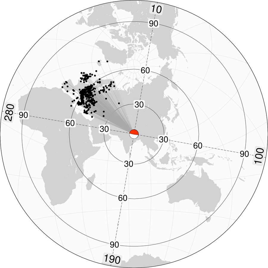
We use P-wave velocity records at the Virtual European Broadband Seismic Network (VEBSN), filtered between 0.5 and 1.0 Hz and between 1.0 and 4.0 Hz.
Signals are realigned according to theoretical arrival time from the USGS epicenter, using multichannel cross-correlation – see Trace alignment.
We use the back projection method described in Satriano et al. (2012).

Station distribution - Stereographic Projection

VEBSN stations used for the back projection analysis.
(click on the images for a larger version)

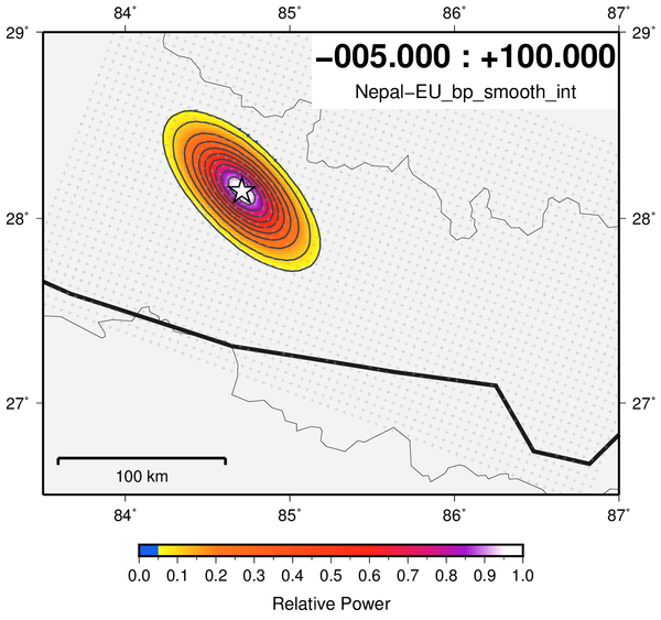
Back projection resolution is estimated by the array response function (ARF), computed at the lowest frequency of the band (0.5 and 1.0 Hz). The ARF allows to correctly evaluate the beam power images obtained from the back projection analysis.
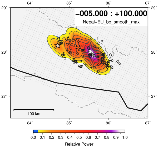
For back projection imaging we use a linear trace stack weighted by trace semblance.

Semblance-weighted linear stack shows unilateral rupturing to the east of the epicenter.

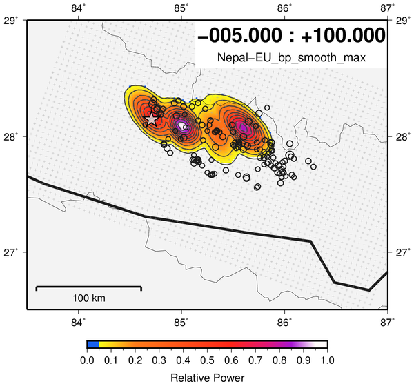
Array response function @0.5Hz Array response function @0.5Hz - Linear stack, semblance weight	Maximum beam power over time @0.5-1.0 Hz Maximum beam power over time @0.5-1.0 Hz
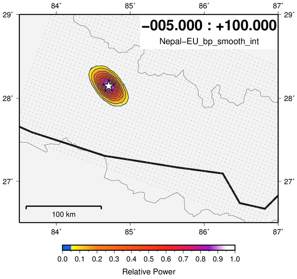
Array response function @1.0Hz Array response function @1.0Hz - Linear stack, semblance weight	Maximum beam power over time @1.0-4.0 Hz Maximum beam power over time @1.0-4.0 Hz

Array response function (left) and maximum beam power over time (right) for semblance-weighted linear stack. The star is the epicenter. Dots are aftershocks, up to May 4, located by NSC.
(click on the images for a larger version)

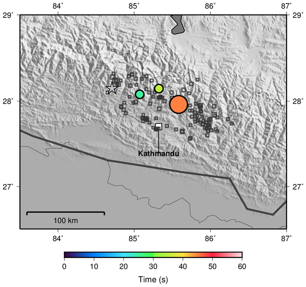
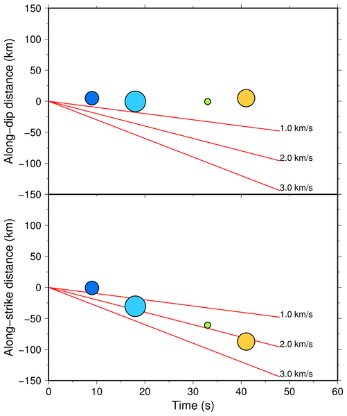
We extract over time local maxima of back projection beam power. These back projection peaks are locations of high-frequency (~0.5 and ~1.0 Hz) coherent energy emitters.
For semblance-weighted linear stack, the circle amplitude is mostly related to the actual signal energy (with some weighting based on coherency).

Rupture propagates unilaterlay to the east. High-frequency emission is to the north of the aftershock area (downdip limit of the coupled interface?). Energy emission is stronger at later stages of the rupture (see also Energy time function and Trace alignment). The last coherent source appears at ~95 km east of the epicenter.

Back projection peaks @0.5-1.0Hz Back projection peaks - Linear stack, semblance weight @0.5-1.0Hz

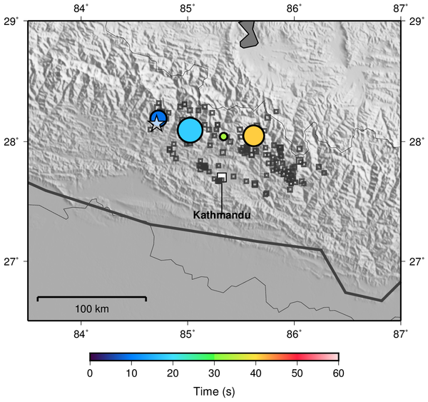
Back projection peaks @1.0-4.0Hz Back projection peaks - Linear stack, semblance weight @1.0-4.0Hz

Time coded back projection peaks for semblance-weighted linear stack. Circle amplitude is proportional to beam power. The star is the epicenter. Squares are aftershocks, up to May 4, located by NSC. The white square indicates the city of Kathmandu.
(click on the images for a larger version)

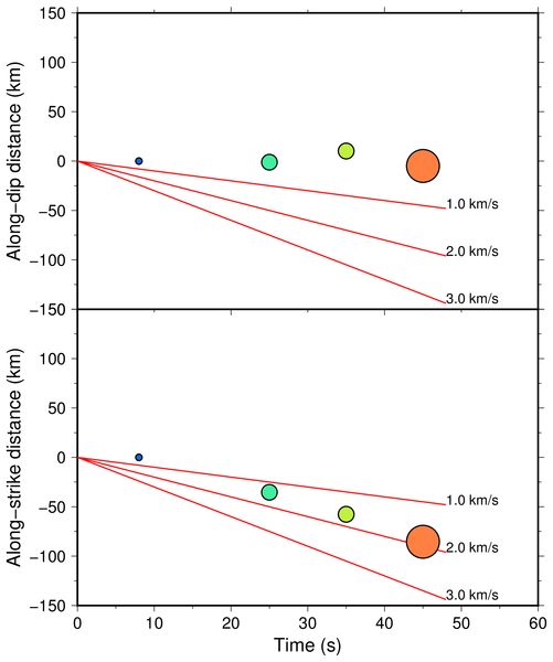
Projected peaks along-strike show coherent sources activating to the east at increasing time with apparent velocity of ~2.0 km/s. Along-dip source position doesn't change significantly with time.

Back projection peaks, projected @0.5-1.0Hz Back projection peaks, projected - Linear stack, semblance weight @0.5-1.0 Hz

Back projection peaks, projected @1.0-4.0 Hz Back projection peaks, projected - Linear stack, semblance weight @1.0-4.0 Hz

Time coded back projection peaks for semblance-weighted linear stack projected along-dip (top) and along-strike (bottom). Zero-distance corresponds to the epicentral location. Circle amplitude is proportional to beam power. Lines indicate reference rupture velocities.
(click on the images for a larger version)

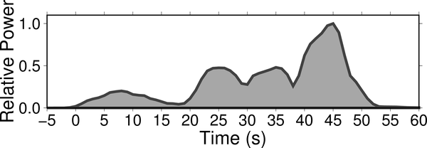
We look at coherent energy release as a function of time by integrating back projection beam power on space at every time step.

Energy release between 0.5 and 1.0 Hz is stronger at later stages of the rupture.
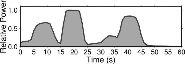
Energy release between 1.0 and 4.0 Hz has strong peaks at 9, 18 and 41s.

Energy time function @0.5-1.0 Hz Energy time function - Linear stack, semblance weight @0.5-1.0 Hz

Energy time function @1.0-4.0 Hz Energy time function - Linear stack, semblance weight @1.0-4.0 Hz

Space-integrated beam power as a function of time for semblance-weighted linear stack.
(click on the images for a larger version)

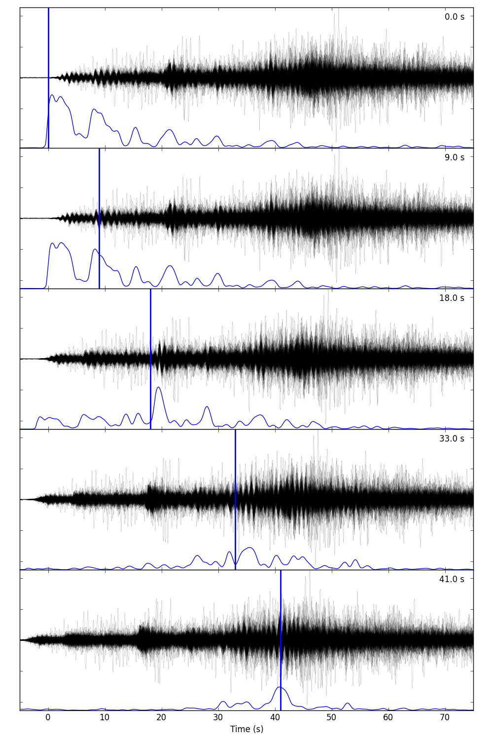
Trace filtered between 0.5 and 1.0 Hz show stronger energy release at later stages of the rupture.
Trace filtered between 1.0 and 4.0 Hz show at least three "sub-events" (0, 9, 18s) with increasing energy and a last coherent source at 41s (stopping phase?).

Trace alignment @0.5-1.0 Hz Trace alignment - Linear stack, semblance weight @0.5-1.0Hz

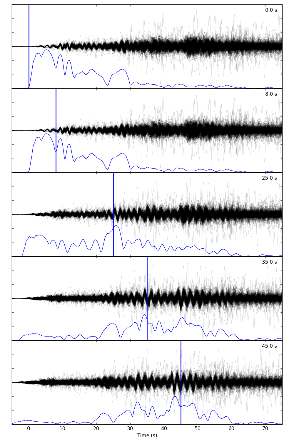
Trace alignment @1.0-4.0 Hz Trace alignment - Linear stack, semblance weight @1.0-4.0Hz

Trace alignment for semblance-weighted linear stack. Top panel is trace alignment according to theoretical arrival time from origin. Following panels show trace alignment corresponding to each of the detected back projection peaks. Blue curve is semblance function. Vertical blue line is the arrival time corresponding to back projection peak.
(click on the images for a larger version)

C. Satriano, E. Kiraly, P. Bernard, J.-P. Vilotte (2012). The 2012 Mw 8.6 Sumatra earthquake: evidence of westward sequential seismic ruptures associated to the reactivation of a N-S ocean fabric, Geophys. Res. Lett., 39(15), L15302, doi 10.1029/2012GL052387.